Articles
Analyzing How Many Space Specific Extension Takes Within a Folder
In today’s digital age, ensuring efficient management of storage space is key to maintaining optimal system performance and avoiding needless clutter. Using SQL queries to assess folder sizes based on file extension is an effective method for pinpointing and managing large files, thus optimizing storage space with precision. This guide demonstrates the power of a structured SQL-like analysis in exposing the distribution of disk space usage among different file types, helping you make informed decisions for data management and storage optimization.
Introduction: The Importance of Efficient Storage Management
The ability to sift through and analyze large datasets with SQL proves invaluable in digital storage management. By executing a specialized SQL-like query, you can obtain detailed insights into how storage space is allocated, particularly useful when optimizing disk space for enhanced system operation. This guide introduces a systematic approach to utilize SQL for examining folder sizes by certain file extensions, emphasizing the need for proactive storage space management.
In-Depth Examination of the SQL Query
select
    Extension,
    Round(Sum(Length) / 1024 / 1024 / 1024, 1) as SpaceOccupiedInGB,
    Count(Extension) as HowManyFiles
from #os.files('C:\Users\{USER}\Downloads', true)
group by Extension
having Round(Sum(Length) / 1024 / 1024 / 1024, 1) > 0
Understanding the #os.files Function
Central to our analysis is the #os.files function. This function acts as a bridge to the filesystem, allowing us to gather file information from a specified directory, such as C:\Users\{USER}\Downloads. Key points include:
- Customization: Adjust the directory path
C:\Users\{USER}\Downloadsby substituting{USER}with your actual username to accurately target the Downloads folder. - Comprehensive Search: By setting the recursive search parameter to
true, you ensure a thorough investigation of the directory and its subdirectories, providing a full overview of its contents.
Decoding File Attributes via SELECT Clause
Extracting essential file attributes, Extension for categorization and Length for size in bytes, furnishes us with a detailed breakdown of storage space distribution among various file types:
- Bytes to Gigabytes Conversion: Converting file sizes from bytes to gigabytes (GB) using
Round(Sum(Length) / 1024 / 1024 / 1024, 1)renders the volume of data comprehensible, making it easier for users to take action.
The Role of GROUP BY and HAVING Clauses
The strategic application of GROUP BY Extension and the HAVING clause to set size thresholds helps focus our disk cleanup efforts by filtering significant space consumers. This targeted filtering by file extension and size equips users to execute disk space recovery with heightened effectiveness.
Interpreting Results and Taking Action
The resulting table displays file extensions along with the corresponding total space taken in GB and file count, facilitating the identification of major storage occupants for potential cleanup or archiving:
| Extension | SpaceOccupiedInGB | HowManyFiles |
|---|---|---|
| .gz | 0.2 | 4 |
| .xz | 20.0 | 13 |
For example, file types such as .xz may disproportionately consume storage space (20 GB), underlining the importance of adopting specific data management strategies.
Expanding Your Disk Space Analysis
I encourage broadening your analysis to encompass various directories or file types, pinpointing primary storage occupiers is always efficient cleanup strategies.
Navigating Permissions and Access
To successfully execute the query, ensure you have the required access permissions for the directory. Addressing any path syntax, permissions, or compatibility concerns is paramount for accessing the desired file information.
Utilizing SQL-like tools for an in-depth disk space analysis furnishes you with critical insights for effective storage management. This guide highlights the pivotal role regular, data-driven disk space reviews play in overall digital housekeeping, aiming to bolster storage optimization and system performance initiatives.
Checking for duplicates within a folder
Detecting duplicates in our file systems is crucial for optimizing storage space, enhancing data organization, and eliminating redundancies that might affect decision-making or data analysis. The tool is excellent at browsing through files and executing complex operations to identify duplicate files with finesse. Let’s delve into a carefully crafted process, highlighting the significance and operations of each step:
- Listing all files: We start by scanning for all files within the target directory and its subdirectories. This fundamental step ensures no file is overlooked in our search for duplicates.
- Grouping by size: Next, we group files by their size, using size as a primary filter to identify potential duplicates. This step focusses our attention on files that might be duplicates, although it’s important to analyze further for accurate identification.
- Quick hashing of partial content: For files of the same size, we examine fragments from different sections (beginning, possibly middle, and end) using cryptographic methods like MD5 or SHA-1. This step filters out files of identical size but different contents, allowing for quick and precise screening.
- Full hashes for suspected duplicates: We intensify our examination for files with matching preliminary hashes by calculating full hashes across their entire content. This step is critical in confirming that only true duplicates, verified through a complete content match, are identified.
Now, let’s automate these steps using SQL:
with PotentialDuplicates as (
    select
        Length,
        Count(Length) as HowManyFiles
    from #os.files('D:\\duplicates', true)
    group by Length
    Having Count(Length) > 1
), QuickHashes as (
    select
        f.FullName as FullName,
        f.Length as Length,
        Md5(
            MergeArrays(
                f.Head(100),
                case when f.Length <= 100 then GetBytes('') else f.GetFileBytes(100, (f.Length / 2) - 50) end,
                case when f.Length <= 100 then GetBytes('') else f.Tail(100) end
            )
        ) as FastHash
    from #os.files('D:\\duplicates', true) f
    inner join PotentialDuplicates p on f.Length = p.Length
), FullHashes as (
    select
        q1.FullName as FirstFileFullName,
        q2.FullName as SecondFileFullName,
        q1.Length as Length,
        q1.FastHash as FirstFastHash,
        q2.FastHash as SecondFastHash,
        (case when q1.FastHash = q2.FastHash then f.Md5File() else 'certainly-not-duplicated' end) as FullHash
    from QuickHashes q1
    inner join QuickHashes q2 on q1.Length = q2.Length and q1.FullName <> q2.FullName
    inner join #os.files('D:\\duplicates', true) f on f.FullName = q1.FullName
)
select
    f.FullHash,
    AggregateValues(f.FirstFileFullName) as Duplicates
from FullHashes f
where f.FullHash <> 'certainly-not-duplicated'
group by f.FullHash
Diving into this SQL script helps us understand the layered strategy:
- PotentialDuplicates CTE: Initiates by grouping files by length to pinpoint those with potential duplicate sizes, starting our duplicate detection.
- QuickHashes CTE: Uses cryptographic hashing to sift through similarly-sized files, identifying unique contents and potential duplicates quickly and accurately.
- FullHashes CTE: Performs a thorough comparison, where calculating the full content hash for potentially identical files ensures that only true duplicates are flagged.
By executing this SQL script, we navigate through levels of analysis, from broad categorization to precise identification. With the results that query provides, we can smartly decide whatever we want to do with the files.
Comparsion of two folders
Imagine you’ve just backed up your important project files to an external hard drive, or you’ve transferred a batch of documents from one computer to another. How can you be sure that all files have been accurately copied without any missing or altered? This scenario underscores the significance of comparing the contents of two folders—a task critical for ensuring data integrity across different storage locations. This article explores two distinct SQL-like methods tailored for this purpose, catering to varying levels of SQL expertise. We introduce an effortless, predefined method using dirscompare for straightforward comparisons, and a more detailed, manual approach for those seeking deeper insights.
Simplified Method using dirscompare: Simplifying Comparisons
Leveraging the dirscompare function offers a direct, efficient method for comparing two directories. This approach abstracts complexities, providing a user-friendly means to quickly identify differences between folder contents.
SELECT
    (
        CASE WHEN SourceFile IS NOT NULL
        THEN SourceFileRelative
        ELSE DestinationFileRelative
        END
    ) AS FullName,
    (
        CASE WHEN State = 'TheSame'
        THEN 'The Same'
        ELSE State
        END
    ) AS Status
FROM #os.dirscompare('E:\DiffDirsTests\A', 'E:\DiffDirsTests\B')
Understanding the dirscompare Function:
- It instantly identifies if files are ‘The Same’, ‘Modified’, added, or removed by evaluating the
State, making it a breeze to check folder synchronization and modifications. - Perfect for scenarios that demand fast and simple comparisons, eliminating the delve into the complexity of data.
Manual Query Design for Folder Comparison: Unveiling Deeper Insights
When deeper analysis is necessary or the dirscompare function doesn’t meet your needs, a manual comparison using crafted queries provides a thorough examination.
WITH filesOfA AS (
    SELECT
        GetRelativePath('E:\DiffDirsTests\A') AS FullName,
        Sha256File() AS ShaedFile
    FROM #os.files('E:\DiffDirsTests\A', true)
), filesOfB AS (
    SELECT
        GetRelativePath('E:\DiffDirsTests\B') AS FullName,
        Sha256File() AS ShaedFile
    FROM #os.files('E:\DiffDirsTests\B', true)
), inBothDirs AS (
    SELECT
        a.FullName AS FullName,
        (
            CASE WHEN a.ShaedFile = b.ShaedFile
            THEN 'The Same'
            ELSE 'Modified'
            END
        ) AS Status
    FROM filesOfA a INNER JOIN filesOfB b ON a.FullName = b.FullName
), inSourceDir AS (
    SELECT
        a.FullName AS FullName,
        'Removed' AS Status
    FROM filesOfA a LEFT OUTER JOIN filesOfB b ON a.FullName = b.FullName
    WHERE b.FullName IS NULL
), inDestinationDir AS (
    SELECT
        b.FullName AS FullName,
        'Added' AS Status
    FROM filesOfA a RIGHT OUTER JOIN filesOfB b ON a.FullName = b.FullName
    WHERE a.FullName IS NULL
)
SELECT
    inBoth.FullName AS FullName,
    inBoth.Status AS Status
FROM inBothDirs inBoth
UNION ALL
SELECT
    inSource.FullName AS FullName,
    inSource.Status AS Status
FROM inSourceDir inSource
UNION ALL
SELECT
    inDest.FullName AS FullName,
    inDest.Status AS Status
FROM inDestinationDir inDest
Step-by-Step Guide to Building Your Query
We will split our challenge into four distinct steps:
- Start with Listing the Files: Begin by itemizing files from each directory, noting their relative paths and generating SHA-256 hashes for a secure comparative basis.
- Identify Identical and Modified Files: Utilize the hash comparison to distinguish identical files and those that have been modified. This step is crucial for tracking synchronization and changes.
- Spot Files Exclusive to Each Folder: This stage is dedicated to detecting files only present in either the source or destination directory, marked as ‘Removed’ or ‘Added.’ Understanding these discrepancies is key to grasping data evolution.
- Compile the Results: The final output merges all findings, presenting a detailed overview of file statuses across directories. This comprehensive perspective aids in grasping modifications and consistency.
By deploying SHA-256 hashing and Common Table Expressions (CTEs), this method showcases high reliability in modification detection and query readability.
Conclusion
Armed with these SQL-like strategies for folder content comparison, you’re well-equipped to handle your analytical needs—whether you require a quick glance or an in-depth exploration. These methods empower you with the capacity to navigate and decipher filesystem modifications efficiently and accurately. Depending on your specific needs, select the most suitable approach to amplify your data management practices.
Generating ranged IP addresses
Recently I stumbled upon a necessity to generate IP ranged addresses.
I was working on allowing developers to use a single self signed certificate across multiple environments we have.
To do so, while generating certificate, there must be a section alt_names that contains IP entries written in such manner
IP.1 = 10.0.12.13
IP.2 = 10.0.12.14
...
IP.N = 10.0.X.Y
It’s necessary to add that asteriks (*) sign is not allowed in certificate so the only option is to propagate the range we have mentioned before.
The problem I had was that I couldn’t assume developers will have assigned static ip in the future so I had to use pregenerated ranges that I would include into certificate.
Based on that I introduce how to generate the range using Musoq.
Let’s look at the query:
select
	Replace(
		Replace(
			Replace('IP.{X}=10.0.{A}.{B}', '{A}', ToString(r1.Value)),
			'{B}',
			ToString(r2.Value)),
		'{X}',
		ToString(RowNumber()))
	from
		#system.range(0, 256) r1 inner join
		#system.range(0, 256) r2 on 1 = 1
and the result it generates:
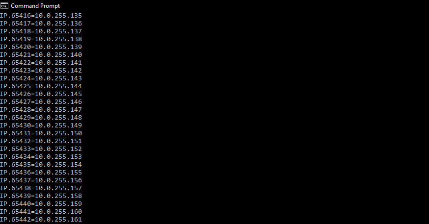
The way how this query works is pretty easy. We just do the cross join of two ranges and for each pair of r1 and r2 replace {A} and {B} from text. The last thing is to just replace {X} with the row number.
That way, we are also able to customize our range with where clause. For example we would mark isles that we are focused on ... where r1.Value > 10 and r1.Value <= 20 and r2.Value > 40 and r2.Value <= 50
Analyzing space consumption on partition with Windows and SQL
Once upon a time in my computer… I faced a problem that appears to all of us from time to time. I was rumming in the system settings and I suddenly realized that my primary partition is almost full. There were only 30 gigabytes left and I really don’t know where all of my empty space disappeared as I haven’t installed anything big lately. To be honest, it’s not that it just disappeared. It was long term process that I was just ignoring for a long period of time. I’m aware of how Windows loves to consume all space left so I decided to analyze it and figure out what those files are and can I delete them?
This is what we want to achieve:
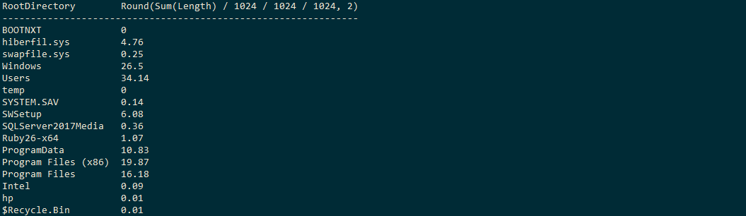
Clear table with listed directories and the space they occupies (including sub directories!). As there is a tremendous amount of files in the file system we need something that does quick overview of where to look for lost space.
It’s my personal preference to continuously go deeper into tree only for that directories that have high level of used space. This way, I can visit only those directories that have something big inside (or aggregated size of files is big) as I don’t want to waste of time to look over lowly occupied folders. Let’s look a query then:
select
	::1 as RootDirectory,
	Round(Sum(Length) / 1024 / 1024 / 1024, 1)
from #os.files('C:/', true)
group by RelativeSubPath(1)
Looks easy, huh? It is so simple because the query does only few things and you don’t see all the underlying operations that evaluator does for you.
First of all, all files are visited on every nested directory of C with C included.
We get the starting location from #os.files('C:/', true).
The literal value true is passed to instruct query evaluator to visit sub directories.
To be precise I have to say we don’t have to be scared that all the files as it visits, will be loaded into memory.
Query evaluator will just read the metadata of the file.
By going further, we would like to visit all of the files in partition and on every of that file apply grouping operator.
In our example, it will work on the result of RelativeSubPath(1).
If you asked me what this method does I would be obligated to say: it gives a relative sub path of the file that is processed.
In fact, the whole method string RelativeSubPath ([InjectSource] ExtendedFileInfo, int nesting) is a shorthand for two different methods:
string SubPath(string directory, int nesting)string GetRelativePath(ExtendedFileInfo fileInfo, string basePath)
Result of that method is string that contains the relative path to one of the main directories we started to traverse from so in our case it will be C:/Some.
Let me explain it on a simple example, if your path is:
C:\Some\Very\Long\Path
and you start from
C:\
then your relative path will be Some\Very\Long\Path.
If your path is the same but you starts from
C:\Some
then your relative path will be Very\Long\Path.
Did you get it? There is still literal argument 1 passed to this method.
With these argument, we can limit the depth of the relative path Some\Very\Long\Path by setting it some numeric.
With argument value 1 we end up with Some, with 2 it’s gonna be Some\Very.
Based on that, we are able to flattening the whole tree to small subset of main directories.
We can match the file from nested directory with the top directory as if it would belong to him directly.
Every single file will belong to a single group - group that describes one of main directories.
Conclusion
I hope it will be usefull you. In the future I will probably write about something more advanced using Musoq. Primarily I will describe my peripeteia with the tool as it is my swiss army knife I use with combination of other tools. If you enjoyed the reading and wants to ask something, please contact me through email or just make an issue within the github project.